Correlated Gaussian Random Variables
Function gnoise1(var,n)                                    // n draws of m-dim vector of corr. noise
	wave var; variable n                               // var must be sym, pos-def. matrix
	variable m=dimsize(var,0)
	MatrixOp /free cholesky=chol(var)                    // compute Cholesky decomposition
	make /d/free/n=(n,m) uncorr=gnoise(1)             // uncorrelated N(0,1) data
	MatrixOp /o corrdat = uncorr x cholesky
End
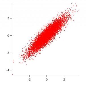
Here is a driver routine to demonstrate how it works (for 2d noise of specified correlation coefficient rho):
Function Demo2d(s1,s2,rho,nsamples,)
	variable s1,s2,rho,nsamples				       // correlation coeff:  -1 < rho < 1
	make /d/o/n=(2,2) var={{s1^2, rho*s1*s2},{rho*s1*s2,s2^2}}	   // make 2x2 covariance matrix
	gnoise1(var,nsamples);		wave corrdat

	Display corrdat[*][1] vs corrdat[*][0]
	ModifyGraph height={Plan,1,left,bottom}, mode=2, lSize=2
End
You can call it with
Demo2d(1,1,0.9,1e4)
and it should look like the attached graph.


Forum

Support

Gallery
Igor Pro 10
Learn More
Igor XOP Toolkit
Learn More
Igor NIDAQ Tools MX
Learn More

It needs to be adapted a bit in this case, as the covariance matrix has NaN entries for the parameters that are being held. The following code snippet takes the fitted coefficients from Funcfit, along with the covariance matrix, and the holdstring (specifying which parameters are being held), and creates 2D wave called M_montecarlo.
This wave has howmany rows, and numpnts(coefs) columns.
Each of the rows contains a set of parameters which could be fed to the fit function used. Futhermore, for a given (parameter) column the mean and standard deviation of that column is equal to the fitted parameter and it's uncertainty. Moreover, different columns possess the correct covariance as specified by the input covariance matrix.
July 14, 2013 at 04:54 pm - Permalink
I couldn't resist the temptation to try it in 3D. The new command line, demo function and Gizmo macro are:
The Gizmo plot should resemble the attached figure. (The Gizmo Macro and figure have been updated to include a display enhancement suggested by WaveMetrics' AG.)
July 17, 2013 at 03:24 am - Permalink