FFT of even-symmetric function yields non-negligible imaginary part


I performed FFT on a cosine function with even symmetricity around zero. Based on the Fourier transform principle, I did not expect any imaginary part in the transformed profile. However, the imaginary part always exists. Do you have any suggestions about what is wrong with my code?
function corr()

	variable xmin = -1
	variable xmax = 1

	make/N=21/O tt

	SetScale/I x, xmin, xmax, tt
	tt = cos(2*pi*x)
	deletePoints 20, 1, tt // delete last point

	FFT/OUT=1/PAD={100000}/DEST=tt_FFT  tt

end
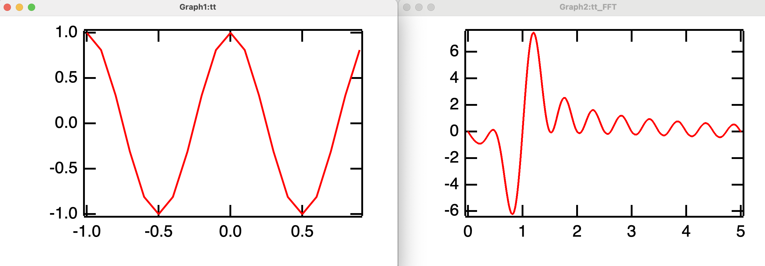
I believe your mistake is to pad using the FFT. You would be better to wrap the function. See the illustration. You have to wrap manually.
Try the function below with variations to npnts and with nopad present or not.
January 18, 2025 at 03:22 pm - Permalink
Hello Maru,
I'd like to focus on a couple of issues that come up in your example:
1. 20 data points over the interval do not provide enough data to approximate the cosine function. All you need to do is check your plot to observe the straight lines and pointy peaks to realize that your input to the FFT is undersampled.
2. As indicated in JJWeimer's post, you have a problem with the boundaries (start and end of the array). Proper padding helps but the padding creates a step transition from the value of the function (~1) to zero. The step does not help your FFT. To resolve this issue you should look at applying a Window function. These are available as an option in the FFT operation.
Based on the syntax you are using, the result of the FFT will always be complex and the imaginary component will not be identically zero. You can investigate the improvements by computing the ratios of the real to the imaginary components as you increase the sampling of the data and apply proper window functions. Remember that the theoretical transform of the cosine consists of a couple of delta functions but you will only see the one on the positive frequency side due to the choice of transform.
AG
January 22, 2025 at 02:58 pm - Permalink
Thank you for the suggestions. The pad was the primary reason for the substantial imaginary part. If I add a pad of the same size to both sides of the cosine profiles, making the function symmetric with the added pads, the imaginary part becomes negligible. Yes, it was not zero yet but reduced to a minimal value.
The non-smooth transition generates many ripples but is not the cause of the imaginary part. The window function did not reduce the imaginary part because the functions were still asymmetric.
January 23, 2025 at 10:51 pm - Permalink
> If I add a pad of the same size to both sides of the cosine profiles, making the function symmetric with the added pads, the imaginary part becomes negligible.
Consider extending the segment with only two cycles by concatenating the same segment a few dozen or more times rather than padding with zeros.
January 24, 2025 at 07:32 am - Permalink