Igor Pro® includes powerful curve fitting features:

• Fit data to built-in and user-defined fitting functions.
• Do linear, polynomial and non-linear regression.
• Virtually unlimited number of fit coefficients in user-defined fitting functions.
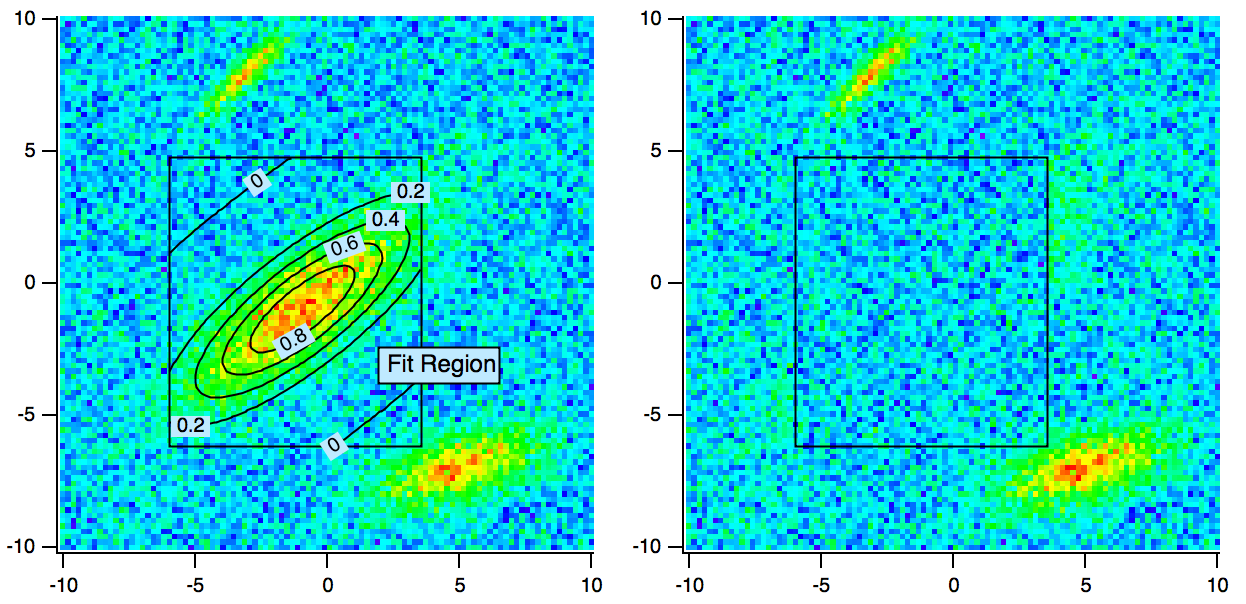
• Virtually unlimited number of independent variables in a Multivariate curve fit (multiple regression).
• Curve fits to data with linear constraints on the fit parameters.
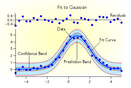
• Automatic calculation of the model curve, curve fit residuals, and confidence and prediction bands. These curves can be automatically added to a graph of your data.
• Optional automatic calculation of confidence limits for fit coefficients.
• Set and hold the value of any fit coefficient.
• Weighted data fitting.
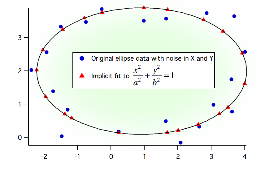
• Errors-in-variables fitting (when you have measurment errors in both X and Y).
• Implicit fits, when your fitting function is in the form f(x,y)=0.
• Curve fit to subsets of your data.
• For simple fits to built-in functions, fit with a single menu selection.
• Fit to sums of fitting functions.
• Follow fit progress with automatic graph updates during iterative fits.
• Fully programmable for repetitive or unusual curve fitting tasks.
• User-defined fits take advantage of multiple processors.
• Programmer support for simultaneous fits using multiple processors.

Packages built on Igor's basic curve fitting capability add functionality:

• Global Analysis
• Peak Analysis

Overview of Curve Fitting

The idea of curve fitting is to find a mathematical model that fits your data. We assume that you have theoretical reasons for picking a function of a certain form. The curve fit finds the specific coefficients (parameters) which make that function match your data as closely as possible. Some people try to use curve fitting to find which of thousands of functions fit their data. Igor is not designed for this purpose.

In curve fitting we have raw data and a function with unknown coefficients. We want to find values for the coefficients such that the function matches the raw data as well as possible. The best values of the coefficients are the ones that minimize the value of Chi-square. Chi-square is defined as:

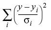
where y is a fitted value (model value) for a given point, y_i is the measured data value for the point and σ_i is an estimate of the standard deviation for y_i.

The simplest case is data fitting to a straight line: y = ax + b, also called "linear regression". Suppose we have a theoretical reason to believe that our data should fall on a straight line. We want to find the coefficients a and b that best match our data. For curve fitting to a straight line or polynomial function, we can find the best-fit coefficients in one step. Igor uses the singular value decomposition algorithm.

Iterative Data Fitting (non-linear least-squares / non-linear regression)

For the other built-in data fitting functions and for user-defined functions, the operation must be iterative. Igor tries various values for the unknown coefficients. For each try, it computes chisquare searching for the coefficient values that yield the minimum value of chi-square.

Initial Guesses

For non-linear least-squares data fitting, Igor uses the Levenberg-Marquardt algorithm to search for the minimum value of chisquare. Chi-square defines a surface in a multidimensional error space. The search process involves starting with an initial guess at the coefficient values. Starting from the initial guesses, Igor searches for the minimum value by travelling down hill from the starting point on the chi-square surface.

We want to find the deepest valley in the chi-square surface. This is a point on the surface where the coefficient values of the fitting function minimize, in the least-squares sense, the difference between the experimental data and fit data (the model). Some curve fitting functions may have only one valley. In this case, when the bottom of the valley is found, the best fit has been found. Some functions, however, may have multiple valleys, places where the fit is better than surrounding values, but it may not be the best fit possible. When Igor finds the bottom of a valley it concludes that the fit is complete even though there may be a deeper valley elsewhere on the surface. Which valley Igor finds first depends on the initial guesses.

For built-in curve fitting functions, you can let Igor automatically set the initial guesses. If this produces unsatisfactory results, you can try manual guesses. For data fitting to user-defined functions you must supply manual guesses.

If you have data containing multiple possibly overlapping peaks, the multi-peak package can automatically analyze your data and generate initial guesses prior to data fitting.

Other data fitting algorithms

Occasionally a user will inquire about other data fitting algorithms such as simulated annealing as an alternative to Levenberg-Marquardt. However, so far we have never seen a case where any algorithm works better than Levenberg-Marquardt. If you know of such an algorithm or data set, please let us know.

Simulated annealing has the appeal of possibly finding a global minimum (the deepest valley in the chi-square surface). It is very time-consuming and by no means guaranteed. You can use Igor's function optimization operation with the simulated annealing option to build a simulated annealing fitter. The standard fitter would then be used to "polish" the result and to provide error estimates.